9  Spatial databases

9.1 Create a connection to DuckDB

library(DBI)
library(duckdb)
library(sf)
library(dplyr)

conn <- dbConnect(duckdb())

9.2 File Path and Database Setup

Here, the code retrieves the file path of a sample GeoPackage file included with the sf package. It also installs and loads the necessary extensions (httpfs and spatial) in DuckDB to handle spatial data.

file <- system.file("gpkg/nc.gpkg", package = "sf")

dbExecute(conn, "INSTALL httpfs; LOAD httpfs; INSTALL spatial; LOAD spatial")

[1] 0

9.3 Creating a Table with Spatial Data

This section constructs a SQL query to create a table (mytable) from the GeoPackage file. It reads the spatial data and converts the geometry column to Well-Known Binary (WKB) format. The query is then executed with the file path bound as a parameter.

query <-
  "
    CREATE OR REPLACE TABLE mytable AS
    SELECT
      *,
      ST_asWKB (geom) AS geom2
    FROM
     ST_Read (?)
  "

stmt <- dbSendStatement(conn, query, params = list(file))
dbGetRowsAffected(stmt)

[1] 100

dbClearResult(stmt)

9.4 Describing the Table

This part describes the structure of the newly created table and lists all tables in the database.

dbSendQuery(conn, "DESCRIBE mytable;") |>
  dbFetch()

column_name	column_type	null	key	default	extra
AREA	DOUBLE	YES	NA	NA	NA
PERIMETER	DOUBLE	YES	NA	NA	NA
CNTY_	DOUBLE	YES	NA	NA	NA
CNTY_ID	DOUBLE	YES	NA	NA	NA
NAME	VARCHAR	YES	NA	NA	NA
FIPS	VARCHAR	YES	NA	NA	NA
FIPSNO	DOUBLE	YES	NA	NA	NA
CRESS_ID	INTEGER	YES	NA	NA	NA
BIR74	DOUBLE	YES	NA	NA	NA
SID74	DOUBLE	YES	NA	NA	NA
NWBIR74	DOUBLE	YES	NA	NA	NA
BIR79	DOUBLE	YES	NA	NA	NA
SID79	DOUBLE	YES	NA	NA	NA
NWBIR79	DOUBLE	YES	NA	NA	NA
geom	GEOMETRY	YES	NA	NA	NA
geom2	WKB_BLOB	YES	NA	NA	NA

dbSendQuery(
  conn,
  "FROM (SUMMARIZE mytable) AS summarized_table WHERE NOT regexp_matches(column_name,'geom')"
) |>
  dbFetch()

column_name	column_type	min	max	approx_unique	avg	std	q25	q50	q75	count	null_percentage
AREA	DOUBLE	0.042	0.241	86	0.12626000000000004	0.04920019298639987	0.091	0.1205	0.1545	100	0
PERIMETER	DOUBLE	0.999	3.64	92	1.6729600000000004	0.4823126510193709	1.323	1.6085	1.863	100	0
CNTY_	DOUBLE	1825.0	2241.0	112	1985.96	106.51664829328959	1901.5	1982.0	2067.5	100	0
CNTY_ID	DOUBLE	1825.0	2241.0	112	1985.96	106.51664829328959	1901.5	1982.0	2067.5	100	0
NAME	VARCHAR	Alamance	Yancey	105	NA	NA	NA	NA	NA	100	0
FIPS	VARCHAR	37001	37199	83	NA	NA	NA	NA	NA	100	0
FIPSNO	DOUBLE	37001.0	37199.0	100	37100.0	58.022983951764346	37050.0	37100.0	37150.0	100	0
CRESS_ID	INTEGER	1	100	96	50.5	29.011491975882013	26	50	76	100	0
BIR74	DOUBLE	248.0	21588.0	101	3299.62	3848.1651269196336	1063.0	2180.5	3957.0	100	0
SID74	DOUBLE	0.0	44.0	24	6.67	7.781167371067509	2.0	4.0	8.5	100	0
NWBIR74	DOUBLE	1.0	8027.0	96	1050.81	1432.9117399353129	180.0	697.5	1172.0	100	0
BIR79	DOUBLE	319.0	30757.0	98	4223.92	5179.458159095233	1308.5	2636.0	4989.0	100	0
SID79	DOUBLE	0.0	57.0	29	8.36	9.431860898041274	2.0	5.0	10.5	100	0
NWBIR79	DOUBLE	3.0	11631.0	101	1352.81	1975.9987511497711	241.0	874.5	1416.5	100	0

9.5 Reading and Converting Spatial Data

Here, the code reads the spatial data from the mytable table, specifying the geometry column (geom2). The result is converted to a tibble and then to an sf object for spatial data manipulation.

res <- st_read(
  conn,
  query =
    "
      SELECT
        *
      FROM
       mytable;
    ",
  geometry_column = "geom2"
) |>
  st_as_sf() |>
  select(-geom) |>
  head()

9.6 Filtering and Plotting Spatial Data

Filter the spatial data based on intersection with a specific point.

tbl(conn, "mytable") |>
  filter(ST_Intersects(geom, "SRID=4326;POINT (-81.5 36.43)")) |>
  select(-contains("geom"))

AREA	PERIMETER	CNTY_	CNTY_ID	NAME	FIPS	FIPSNO	CRESS_ID	BIR74	SID74	NWBIR74	BIR79	SID79	NWBIR79
0.114	1.442	1825	1825	Ashe	37009	37009	5	1091	1	10	1364	0	19

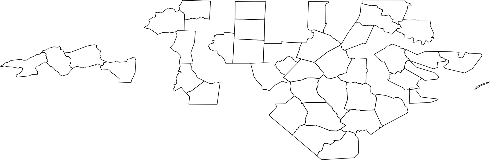
9.7 Filter by Area and Plot

Filter the spatial data based on area greater than 0.14 and plot the results.

res <- tbl(conn, "mytable") |>
  filter(ST_Area(geom) > 0.14) |>
  collect() |>
  st_as_sf()

wkbType: 67108864

plot(st_geometry(res), lwd = 0.5)