3 HE5 format

This section demonstrates how to access and visualize sea ice concentration data stored in HE5 files, focusing on data from the AMSR-E/AMSR2 Unified L3 Daily 12.5 km dataset. We’ll use R along with the gdalraster, stars, terra, and sf packages.

Disclaimer

The code below is largely based/copied on the work of mdsumner.

library(gdalraster)
library(stars)
library(terra)

file <- here::here("data", "AMSR_U2_L3_SeaIce12km_B04_20140314.he5")

The code leverages the NetCDF interface to access subdatasets within the HE5 file. This allows us to access the geolocation arrays, which is crucial for proper spatial referencing.

sub <- paste0("NetCDF:", file, ":")
sds <- gdal_subdatasets(sub)

sf::gdal_utils("info", unlist(sds)[[30L]])

Driver: netCDF/Network Common Data Format
Files: /media/LaCie16TB/work/projects/documentation/read_rs_product/data/AMSR_U2_L3_SeaIce12km_B04_20140314.he5
Size is 608, 896
Metadata:
  /HDFEOS INFORMATION/NC_GLOBAL#HDFEOSVersion=HDFEOS_5.1.15
  /HDFEOS/GRIDS/NpPolarGrid12km/Data Fields/SI_12km_NH_ICECON_DAY#comment=data value meaning: 0 -- Open Water, 110 -- missing/not calculated, 120 -- Land
  /HDFEOS/GRIDS/NpPolarGrid12km/Data Fields/SI_12km_NH_ICECON_DAY#coordinates=lon lat
  /HDFEOS/GRIDS/NpPolarGrid12km/Data Fields/SI_12km_NH_ICECON_DAY#long_name=Sea ice concentration daily average
  /HDFEOS/GRIDS/NpPolarGrid12km/Data Fields/SI_12km_NH_ICECON_DAY#units=percent
  NC_GLOBAL#Conventions=CF-1.6
  NC_GLOBAL#history=This version of the Sea Ice processing code contains updates provided by the science team on September 16, 2019. For details on these updates, see the release notes provided in the DAP.
  NC_GLOBAL#institution=NASA's AMSR Science Investigator-led Processing System (SIPS)
  NC_GLOBAL#references=Please cite these data as: Markus, T., J. C. Comiso, and W. N. Meier. 2018. AMSR-E/AMSR2 Unified L3 Daily 12.5 km Brightness Temperatures, Sea Ice Concentration, Motion & Snow Depth Polar Grids, Version 1. [Indicate subset used]. Boulder, Colorado USA. NASA National Snow and Ice Data Center Distributed Active Archive Center. doi: https://doi.org/10.5067/RA1MIJOYPK3P.
  NC_GLOBAL#source=satellite observation
  NC_GLOBAL#title=AMSR-E/AMSR2 Unified L3 Daily 12.5 km Brightness Temperatures, Sea Ice Concentration, Motion & Snow Depth Polar Grids
Geolocation:
  SRS=GEOGCS["WGS 84",DATUM["WGS_1984",SPHEROID["WGS 84",6378137,298.257223563,AUTHORITY["EPSG","7030"]],AUTHORITY["EPSG","6326"]],PRIMEM["Greenwich",0,AUTHORITY["EPSG","8901"]],UNIT["degree",0.0174532925199433,AUTHORITY["EPSG","9122"]],AXIS["Latitude",NORTH],AXIS["Longitude",EAST],AUTHORITY["EPSG","4326"]]
  X_DATASET=NETCDF:"/media/LaCie16TB/work/projects/documentation/read_rs_product/data/AMSR_U2_L3_SeaIce12km_B04_20140314.he5":/HDFEOS/GRIDS/NpPolarGrid12km/lon
  X_BAND=1
  Y_DATASET=NETCDF:"/media/LaCie16TB/work/projects/documentation/read_rs_product/data/AMSR_U2_L3_SeaIce12km_B04_20140314.he5":/HDFEOS/GRIDS/NpPolarGrid12km/lat
  Y_BAND=1
  PIXEL_OFFSET=0
  PIXEL_STEP=1
  LINE_OFFSET=0
  LINE_STEP=1
  GEOREFERENCING_CONVENTION=PIXEL_CENTER
Corner Coordinates:
Upper Left  (    0.0,    0.0)
Lower Left  (    0.0,  896.0)
Upper Right (  608.0,    0.0)
Lower Right (  608.0,  896.0)
Center      (  304.0,  448.0)
Band 1 Block=608x1 Type=Int32, ColorInterp=Undefined
  Unit Type: percent
  Metadata:
    NETCDF_VARNAME=SI_12km_NH_ICECON_DAY
    coordinates=lon lat
    long_name=Sea ice concentration daily average
    units=percent
    comment=data value meaning: 0 -- Open Water, 110 -- missing/not calculated, 120 -- Land

The data needs to be transformed to a standard coordinate reference system (CRS). EPSG:3411 (NSIDC Sea Ice Polar Stereographic North) is commonly used for Northern Hemisphere sea ice data. The gdal_utils() function warps the data to this CRS and saves it to a temporary VRT (Virtual Raster) file. VRT files are useful because they act as a pointer to the original data without duplicating it, and allow for on-the-fly transformations.

dsn <- "/vsimem/temp.vrt"

sf::gdal_utils(
  "warp",
  unlist(sds)[[30L]],
  dsn,
  options = c("-t_srs", "EPSG:3411", "-overwrite")
)

The rast() function from the terra package is used to read the VRT file and create a SpatRaster object. This object contains the sea ice concentration data, which can be visualized using the plot() function.

r <- rast(dsn)
r

class       : SpatRaster 
dimensions  : 897, 608, 1  (nrow, ncol, nlyr)
resolution  : 12499.99, 12499.99  (x, y)
extent      : -3850009, 3749985, -5356238, 5856254  (xmin, xmax, ymin, ymax)
coord. ref. : NSIDC Sea Ice Polar Stereographic North (EPSG:3411) 
source      : temp.vrt 
name        : temp

plot(r)

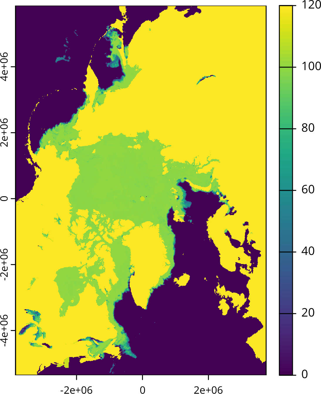
3.1 Using `terra` directly

Warning

Reading data from HE5 files using the terra package may not always work correctly, and you might encounter the error message “cannot find the spatial extent.” If this happens, you can use the gdalraster package to read the data and then convert it to a SpatRaster object (as seen above).

To read data directly from an HE5 file with terra, ensure that terra is built with recent versions of the GDAL and PROJ libraries. Note that compatibility with GDAL v3.9.x is unlikely.

The installed version of gdal can be checked with the following command:

gdalinfo --version

GDAL 3.10.1, released 2025/01/08 (debug build)

If you have a recent version of gdal, you read the data directly from the HE5 file with the terra package.

var_names <- describe(file, sds = TRUE)

head(var_names)

id	name	var	desc	nrow	ncol	nlyr
1	HDF5:“/media/LaCie16TB/work/projects/documentation/read_rs_product/data/AMSR_U2_L3_SeaIce12km_B04_20140314.he5”://HDFEOS/GRIDS/NpPolarGrid12km/Data_Fields/SI_12km_NH_18H_ASC	//HDFEOS/GRIDS/NpPolarGrid12km/Data_Fields/SI_12km_NH_18H_ASC	[896x608] //HDFEOS/GRIDS/NpPolarGrid12km/Data_Fields/SI_12km_NH_18H_ASC (32-bit integer)	896	608	1
2	HDF5:“/media/LaCie16TB/work/projects/documentation/read_rs_product/data/AMSR_U2_L3_SeaIce12km_B04_20140314.he5”://HDFEOS/GRIDS/NpPolarGrid12km/Data_Fields/SI_12km_NH_18H_DAY	//HDFEOS/GRIDS/NpPolarGrid12km/Data_Fields/SI_12km_NH_18H_DAY	[896x608] //HDFEOS/GRIDS/NpPolarGrid12km/Data_Fields/SI_12km_NH_18H_DAY (32-bit integer)	896	608	1
3	HDF5:“/media/LaCie16TB/work/projects/documentation/read_rs_product/data/AMSR_U2_L3_SeaIce12km_B04_20140314.he5”://HDFEOS/GRIDS/NpPolarGrid12km/Data_Fields/SI_12km_NH_18H_DSC	//HDFEOS/GRIDS/NpPolarGrid12km/Data_Fields/SI_12km_NH_18H_DSC	[896x608] //HDFEOS/GRIDS/NpPolarGrid12km/Data_Fields/SI_12km_NH_18H_DSC (32-bit integer)	896	608	1
4	HDF5:“/media/LaCie16TB/work/projects/documentation/read_rs_product/data/AMSR_U2_L3_SeaIce12km_B04_20140314.he5”://HDFEOS/GRIDS/NpPolarGrid12km/Data_Fields/SI_12km_NH_18V_ASC	//HDFEOS/GRIDS/NpPolarGrid12km/Data_Fields/SI_12km_NH_18V_ASC	[896x608] //HDFEOS/GRIDS/NpPolarGrid12km/Data_Fields/SI_12km_NH_18V_ASC (32-bit integer)	896	608	1
5	HDF5:“/media/LaCie16TB/work/projects/documentation/read_rs_product/data/AMSR_U2_L3_SeaIce12km_B04_20140314.he5”://HDFEOS/GRIDS/NpPolarGrid12km/Data_Fields/SI_12km_NH_18V_DAY	//HDFEOS/GRIDS/NpPolarGrid12km/Data_Fields/SI_12km_NH_18V_DAY	[896x608] //HDFEOS/GRIDS/NpPolarGrid12km/Data_Fields/SI_12km_NH_18V_DAY (32-bit integer)	896	608	1
6	HDF5:“/media/LaCie16TB/work/projects/documentation/read_rs_product/data/AMSR_U2_L3_SeaIce12km_B04_20140314.he5”://HDFEOS/GRIDS/NpPolarGrid12km/Data_Fields/SI_12km_NH_18V_DSC	//HDFEOS/GRIDS/NpPolarGrid12km/Data_Fields/SI_12km_NH_18V_DSC	[896x608] //HDFEOS/GRIDS/NpPolarGrid12km/Data_Fields/SI_12km_NH_18V_DSC (32-bit integer)	896	608	1

layer <- var_names[["var"]][grepl("SI_12km_NH_ICECON_DAY", var_names[["var"]], fixed = TRUE)]

layer

[1] "//HDFEOS/GRIDS/NpPolarGrid12km/Data_Fields/SI_12km_NH_ICECON_DAY"

ice_layer <- rast(file, subds = layer)

ice_layer

class       : SpatRaster 
dimensions  : 896, 608, 1  (nrow, ncol, nlyr)
resolution  : 12500, 12500  (x, y)
extent      : -3850000, 3750000, -5350000, 5850000  (xmin, xmax, ymin, ymax)
coord. ref. : +proj=stere +lat_0=90 +lat_ts=70 +lon_0=-45 +x_0=0 +y_0=0 +R=6378273 +units=m +no_defs 
source      : AMSR_U2_L3_SeaIce12km_B04_20140314.he5://SI_12km_NH_ICECON_DAY 
varname     : SI_12km_NH_ICECON_DAY 
name        : SI_12km_NH_ICECON_DAY

Why are the dimensions different?

dim(r)

[1] 897 608   1

dim(ice_layer)

[1] 896 608   1

plot(ice_layer)

3.1 Using terra directly

3.1 Using `terra` directly