2  HDF4 format

library(terra)

2.1 NetCDF (Network Common Data Form)

Layers in the file can be listed using the nc_open() function:

file <- here::here("data", "avhrr-only-v2.20160503.nc")

2.1.1 Open NetCDF file using rast()

The terra package provides an alternative method to work with NetCDF files. This creates a SpatRaster object, which is more memory-efficient for large datasets.

To see which layers are available in the file, use the describe() function. Note the var column in the output:

describe(file, sds = TRUE)

id	name	var	desc	nrow	ncol	nlyr
1	NETCDF:“/media/LaCie16TB/work/projects/documentation/read_rs_product/data/avhrr-only-v2.20160503.nc”:sst	sst	[1x1x720x1440] sst (16-bit integer)	720	1440	1
2	NETCDF:“/media/LaCie16TB/work/projects/documentation/read_rs_product/data/avhrr-only-v2.20160503.nc”:anom	anom	[1x1x720x1440] anom (16-bit integer)	720	1440	1
3	NETCDF:“/media/LaCie16TB/work/projects/documentation/read_rs_product/data/avhrr-only-v2.20160503.nc”:err	err	[1x1x720x1440] err (16-bit integer)	720	1440	1
4	NETCDF:“/media/LaCie16TB/work/projects/documentation/read_rs_product/data/avhrr-only-v2.20160503.nc”:ice	ice	[1x1x720x1440] ice (16-bit integer)	720	1440	1

This file contains four layers: sst, anom, err, and ice. They can be opened using the rast() function using the lyrs or subds argument.

Note

TODO: Explain the difference between lyrs and subds.

2.1.1.1 Open a specific layer using lyrs

# To open the sst layer
sst_layer <- rast(paste0("NETCDF:", file, ":sst"))

# To open the anom layer
anom_layer <- rast(paste0("NETCDF:", file, ":anom"))

# To open the err layer
err_layer <- rast(paste0("NETCDF:", file, ":err"))

# To open the ice layer
ice_layer <- rast(paste0("NETCDF:", file, ":ice"))

2.1.1.2 Open a specific layer using subds

# To open the sst layer
sst_layer <- rast(file, subds = "sst")

# To open the anom layer
anom_layer <- rast(file, subds = "anom")

# To open the err layer
err_layer <- rast(file, subds = "err")

# Open the ice layer
ice_layer <- rast(file, subds = "ice")

2.1.2 Plotting

We can visualize the layers using the plot() function:

par(mfrow = c(2L, 2L))
plot(sst_layer, main = "SST")
plot(anom_layer, main = "Anomaly")
plot(err_layer, main = "Error")
plot(ice_layer, main = "Ice")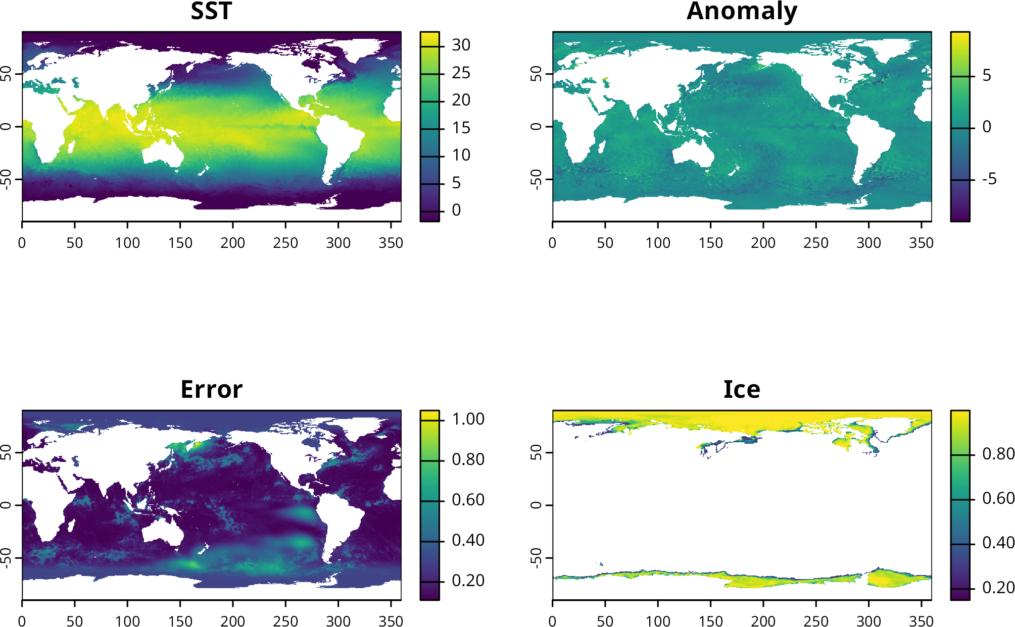

It looks like the raster is rotated. We can rotate it back with the rotate() function:

sst_layer <- rotate(sst_layer)

plot(sst_layer)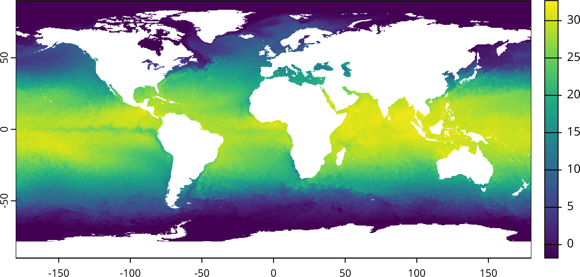

Converting to a data frame can be useful for certain types of analysis or visualization, but be cautious with large datasets as this can be memory-intensive.

df <- as.data.frame(sst_layer)

head(df)

sst_zlev=0
-1.7
-1.7
-1.7
-1.7
-1.7
-1.7