6 Filtering spatial data

library(sf)
library(DBI)
library(duckdb)
library(ggplot2)
library(rnaturalearth)
library(rnaturalearthdata)

In this tutorial, we will explore different methods to filter spatial data using the sf package in R. We will use the Canadian Wind Turbine Database as our example dataset.

6.1 Filtering spatial data with `sf`

The Canadian Wind Turbine Database contains the geographic location and key technology details for wind turbines installed in Canada.

# URL to the wind turbine database
url <- "/vsizip//vsicurl/https://ftp.cartes.canada.ca/pub/nrcan_rncan/Wind-energy_Energie-eolienne/wind_turbines_database/wind_turbine_database_en.gdb.zip"

# List layers in the dataset
st_layers(url)

name	geomtype	driver	features	fields	crs
wind_turbine	Point	OpenFileGDB	7578	17	NAD83 / Canada Atlas Lambert , PROJCRS[“NAD83 / Canada Atlas Lambert”,

BASEGEOGCRS["NAD83",
    DATUM["North American Datum 1983",
        ELLIPSOID["GRS 1980",6378137,298.257222101,
            LENGTHUNIT["metre",1]]],
    PRIMEM["Greenwich",0,
        ANGLEUNIT["degree",0.0174532925199433]],
    ID["EPSG",4269]],
CONVERSION["Canada Atlas Lambert",
    METHOD["Lambert Conic Conformal (2SP)",
        ID["EPSG",9802]],
    PARAMETER["Latitude of false origin",49,
        ANGLEUNIT["degree",0.0174532925199433],
        ID["EPSG",8821]],
    PARAMETER["Longitude of false origin",-95,
        ANGLEUNIT["degree",0.0174532925199433],
        ID["EPSG",8822]],
    PARAMETER["Latitude of 1st standard parallel",49,
        ANGLEUNIT["degree",0.0174532925199433],
        ID["EPSG",8823]],
    PARAMETER["Latitude of 2nd standard parallel",77,
        ANGLEUNIT["degree",0.0174532925199433],
        ID["EPSG",8824]],
    PARAMETER["Easting at false origin",0,
        LENGTHUNIT["metre",1],
        ID["EPSG",8826]],
    PARAMETER["Northing at false origin",0,
        LENGTHUNIT["metre",1],
        ID["EPSG",8827]]],
CS[Cartesian,2],
    AXIS["(E)",east,
        ORDER[1],
        LENGTHUNIT["metre",1]],
    AXIS["(N)",north,
        ORDER[2],
        LENGTHUNIT["metre",1]],
USAGE[
    SCOPE["Transformation of coordinates at 5m level of accuracy."],
    AREA["Canada - onshore and offshore - Alberta; British Columbia; Manitoba; New Brunswick; Newfoundland and Labrador; Northwest Territories; Nova Scotia; Nunavut; Ontario; Prince Edward Island; Quebec; Saskatchewan; Yukon."],
    BBOX[38.21,-141.01,86.46,-40.73]],
ID["EPSG",3978]] |

# Read the entire dataset
pts <- read_sf(url)

# Load and transform Canada map
canada <- ne_countries(
  scale = "medium",
  returnclass = "sf",
  country = "Canada"
) |>
  st_transform(crs = "EPSG:3978")

# Plot the map with wind turbine points
ggplot() +
  geom_sf(data = canada) +
  geom_sf(data = pts, color = "red", size = 0.5)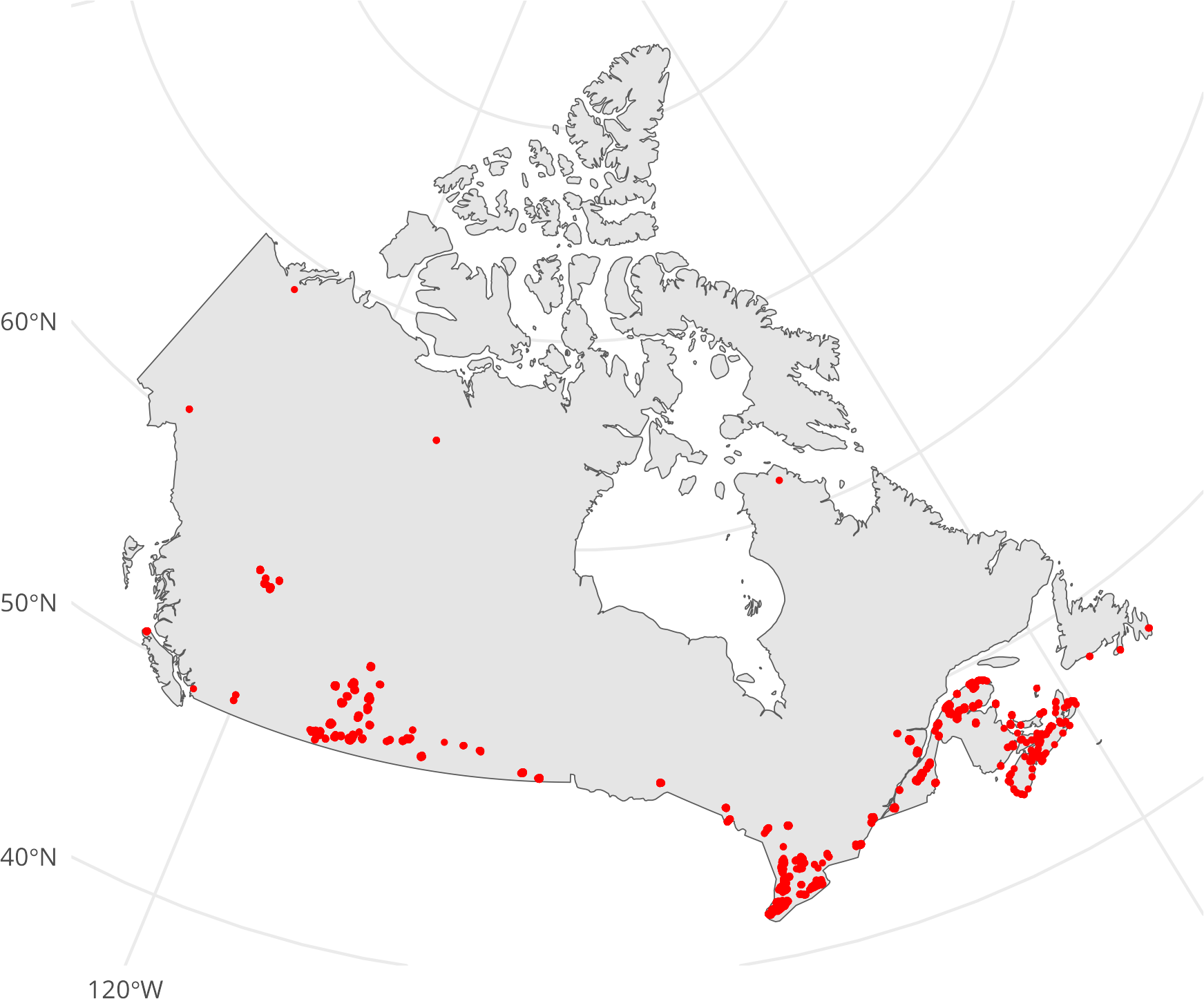

6.2 Filtering spatial data with a bounding box

To avoid loading the entire dataset into memory, we can filter the data using a bounding box. This is particularly useful when working with large datasets. We can leverage the wkt_filter argument to filter spatial data and reduce the amount of data loaded into memory.

# Read and transform the area of interest
area <- read_sf(here::here("data", "area.geojson")) |>
  st_transform(crs = st_crs(pts))

# Plot the map with the area of interest
ggplot() +
  geom_sf(data = canada) +
  geom_sf(data = area, color = "blue", fill = NA, linewidth = 1L) +
  geom_sf(data = pts, color = "red", size = 0.5)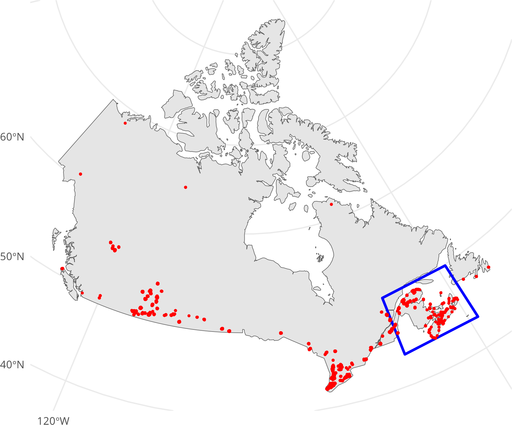

Instead of loading the entire dataset into memory, we can filter the data using a bounding box.

# Convert the area geometry to WKT
wkt <- area |>
  st_geometry() |>
  st_as_text()

# Read the filtered dataset using the bounding box
filtered <- read_sf(url, wkt_filter = wkt)
filtered[["Notes"]] <- NULL


# Plot the filtered data
ggplot() +
  geom_sf(data = canada) +
  geom_sf(data = area, color = "blue", fill = NA, linewidth = 1L) +
  geom_sf(data = filtered, color = "red", size = 0.5)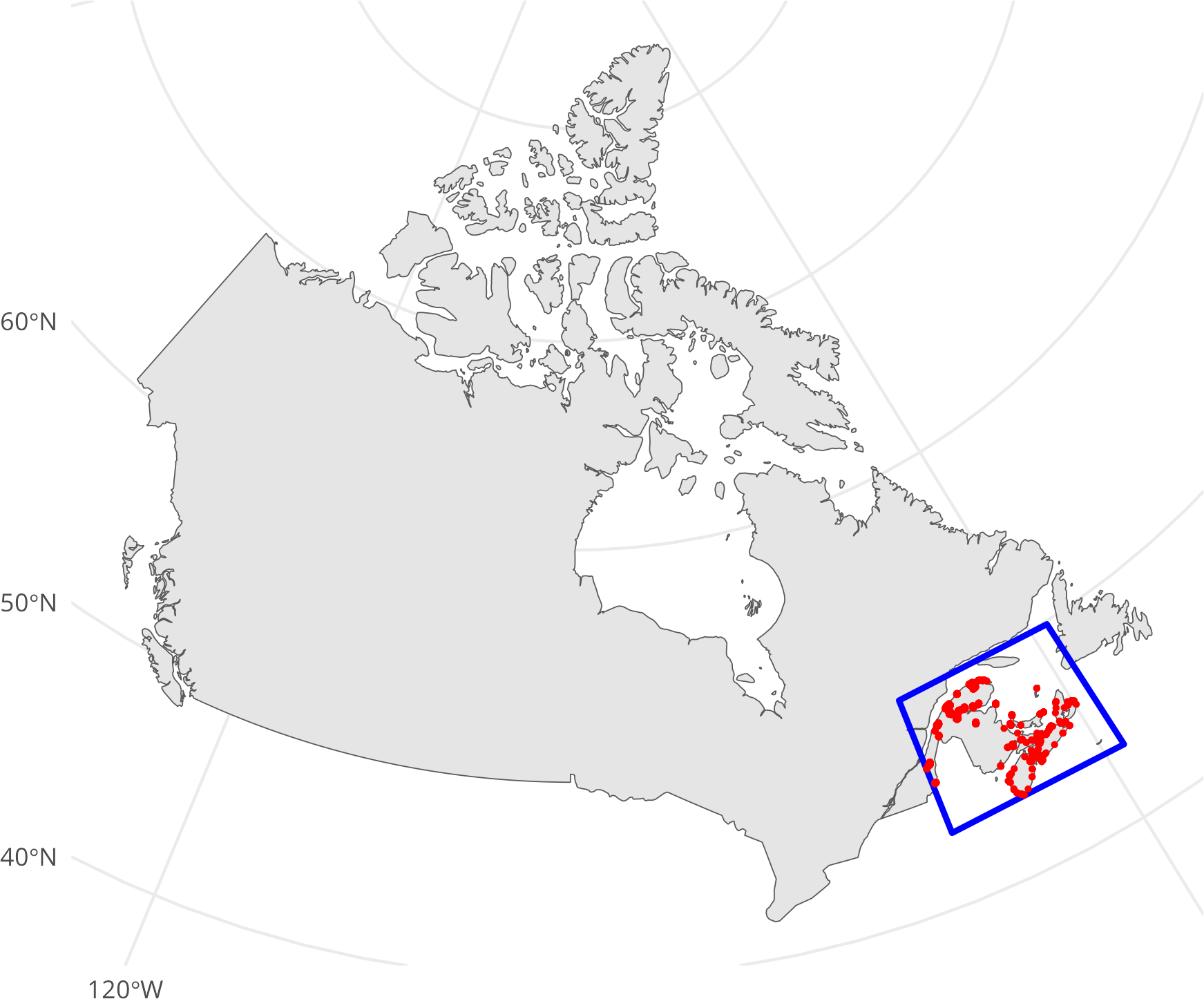

# Display the number of rows and the first few rows of the filtered data
nrow(filtered)

[1] 2032

head(filtered)

Province_Territory	Project_Name	Total_Project_Capacity_MW	Turbine_Identifier	Turbine_Number	Turbine_Number_in_Project	Turbine_Rated_Capacity_kW	Rotor_Diameter_m	Hub_Height_m	Manufacturer	Model	Commissioning	Latitude	Longitude	Data_Sources	Basemap	Shape
New Brunswick	Burchill	42	BRH1	1	1/10	4200	141	135	Enercon	E141-4.2	2023	45.15949	-66.19081	[70], [71], [910]	ESRI	POINT (2225020 82296.21)
New Brunswick	Burchill	42	BRH2	2	2/10	4200	141	135	Enercon	E141-4.2	2023	45.16434	-66.19718	[70], [71], [910]	ESRI	POINT (2224322 82566.09)
New Brunswick	Burchill	42	BRH3	3	3/10	4200	141	135	Enercon	E141-4.2	2023	45.16875	-66.20070	[70], [71], [910]	ESRI	POINT (2223851 82890.97)
New Brunswick	Burchill	42	BRH4	4	4/10	4200	141	135	Enercon	E141-4.2	2023	45.17307	-66.20036	[70], [71], [910]	ESRI	POINT (2223662 83342.02)
New Brunswick	Burchill	42	BRH5	5	5/10	4200	141	135	Enercon	E141-4.2	2023	45.17834	-66.19340	[70], [71], [910]	ESRI	POINT (2223902 84120.34)
New Brunswick	Burchill	42	BRH6	6	6/10	4200	141	135	Enercon	E141-4.2	2023	45.18281	-66.18900	[70], [71], [910]	ESRI	POINT (2223997 84728.45)

6.3 Refining the filter with a user-defined SQL query

We can further refine our filter by using a user-defined query. For example, we can filter the wind turbines based on their rated capacity.

# Display the range of turbine capacities
range(filtered[["Turbine_Rated_Capacity__kW_"]])

[1]    0 4200

To refine the filter, we can use a custom query to select only the wind turbines with a rated capacity greater than 4000 kW. First, we need to identify the layer name to use in the SQL query.

# List layers in the dataset
st_layers(url)

name	geomtype	driver	features	fields	crs
wind_turbine	Point	OpenFileGDB	7578	17	NAD83 / Canada Atlas Lambert , PROJCRS[“NAD83 / Canada Atlas Lambert”,

BASEGEOGCRS["NAD83",
    DATUM["North American Datum 1983",
        ELLIPSOID["GRS 1980",6378137,298.257222101,
            LENGTHUNIT["metre",1]]],
    PRIMEM["Greenwich",0,
        ANGLEUNIT["degree",0.0174532925199433]],
    ID["EPSG",4269]],
CONVERSION["Canada Atlas Lambert",
    METHOD["Lambert Conic Conformal (2SP)",
        ID["EPSG",9802]],
    PARAMETER["Latitude of false origin",49,
        ANGLEUNIT["degree",0.0174532925199433],
        ID["EPSG",8821]],
    PARAMETER["Longitude of false origin",-95,
        ANGLEUNIT["degree",0.0174532925199433],
        ID["EPSG",8822]],
    PARAMETER["Latitude of 1st standard parallel",49,
        ANGLEUNIT["degree",0.0174532925199433],
        ID["EPSG",8823]],
    PARAMETER["Latitude of 2nd standard parallel",77,
        ANGLEUNIT["degree",0.0174532925199433],
        ID["EPSG",8824]],
    PARAMETER["Easting at false origin",0,
        LENGTHUNIT["metre",1],
        ID["EPSG",8826]],
    PARAMETER["Northing at false origin",0,
        LENGTHUNIT["metre",1],
        ID["EPSG",8827]]],
CS[Cartesian,2],
    AXIS["(E)",east,
        ORDER[1],
        LENGTHUNIT["metre",1]],
    AXIS["(N)",north,
        ORDER[2],
        LENGTHUNIT["metre",1]],
USAGE[
    SCOPE["Transformation of coordinates at 5m level of accuracy."],
    AREA["Canada - onshore and offshore - Alberta; British Columbia; Manitoba; New Brunswick; Newfoundland and Labrador; Northwest Territories; Nova Scotia; Nunavut; Ontario; Prince Edward Island; Quebec; Saskatchewan; Yukon."],
    BBOX[38.21,-141.01,86.46,-40.73]],
ID["EPSG",3978]] |

We can use wind_turbine as the layer name in the custom query.

# Read the filtered dataset with a custom query
high_capacity <- read_sf(
  url,
  wkt_filter = wkt,
  query = "SELECT * FROM wind_turbine WHERE Turbine_Rated_Capacity__kW_ > 4000"
)

high_capacity[["Notes"]] <- NULL

# Display the number of rows and the first few rows of the high capacity data
nrow(high_capacity)

[1] 10

# Plot the high capacity turbines
ggplot() +
  geom_sf(data = canada) +
  geom_sf(data = area, color = "blue", fill = NA, linewidth = 1L) +
  geom_sf(data = high_capacity, color = "red", size = 0.5)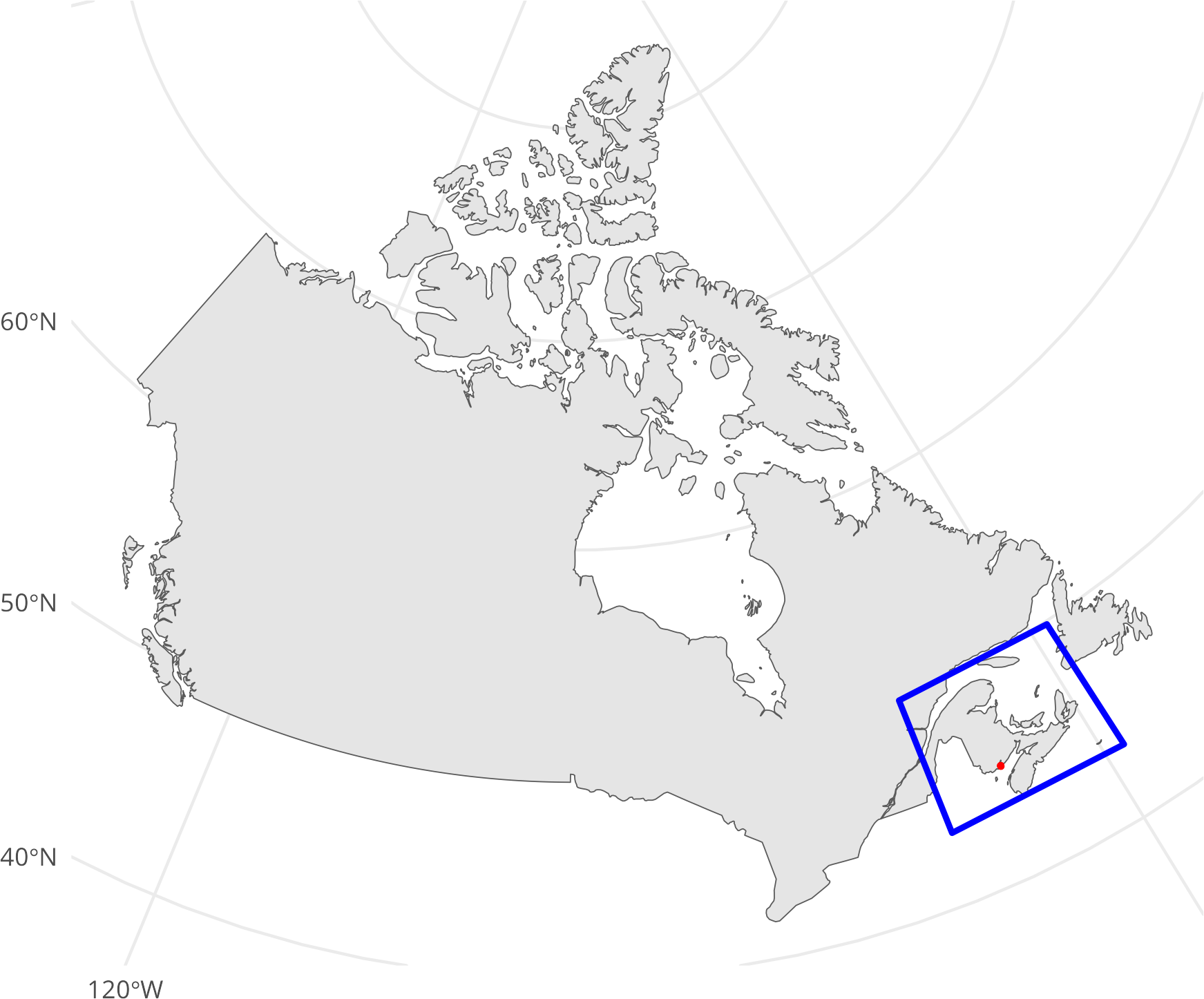

6.4 Filtering spatial data with DuckDB

In this section, we will demonstrate how to filter spatial data using DuckDB. DuckDB is an embedded analytical database that supports spatial extensions.

# Connect to DuckDB
conn <- dbConnect(duckdb())

# Install and load the spatial extension
dbSendQuery(conn, "INSTALL spatial;")
dbSendQuery(conn, "LOAD spatial;")

# Create a table with spatial data filtered by a bounding box
dbSendQuery(
  conn,
  "
  CREATE
  OR REPLACE TABLE t AS
  SELECT
   *,
   ST_asWKB(geom) AS geometry
  FROM
   ST_Read('/vsis3/spatial-playground/gmw_v3.fgb', spatial_filter_box = {'min_x' : - 30, 'min_y' : 0, 'max_x' : - 50, 'max_y' : 45});
  "
)

# Read the filtered data from DuckDB
read_sf(conn, query = "SELECT * FROM t", geometry_column = "geometry")

# Read the filtered data with an additional computed area column
read_sf(
  conn,
  query = "SELECT *, ST_Area(geom) as area1 FROM t",
  geometry_column = "geometry"
) |>
  mutate(area2 = st_area(geometry), .after = area1)

6.1 Filtering spatial data with sf

6.2 Filtering spatial data with a bounding box

6.3 Refining the filter with a user-defined SQL query

6.4 Filtering spatial data with DuckDB

6.1 Filtering spatial data with `sf`