1  Binary format

library(terra)

1.1 NSIDC binary data

Binary data is a format where information is stored in a sequence of bytes, representing data in its most basic form without any text-based structure. This format is efficient for storage and quick to read programmatically, but it’s not human-readable without proper interpretation. In the case of scientific datasets like sea ice concentration, binary formats were often used to minimize file size and optimize data processing speed.

Note

Version 1 of the NSIDC-0081 sea ice concentration dataset is available in binary format but is no longer active. The current version (Version 2) is in NetCDF format.

Based on the documentation, the binary files can be read using the following code:

sic <- readBin(
  here::here("data", "nsidc", "nt_20171002_f17_v1.1_n.bin"),
  what = "integer",
  n = 304L * 448L,
  size = 1L,
  signed = FALSE
)


lat <- readBin(
  here::here("data", "nsidc", "psn25lats_v3.dat"),
  what = "integer",
  n = 304L * 448L,
  size = 4L,
  signed = TRUE
)

lon <- readBin(
  here::here("data", "nsidc", "psn25lons_v3.dat"),
  what = "integer",
  n = 304L * 448L,
  size = 4L,
  signed = TRUE
)

We can construct a data frame from the latitude, longitude, and sea ice concentration data:

df <- data.frame(lat = lat / 100000L, lon = lon / 100000L, sic = sic)

head(df)

lat	lon	sic
31.10267	168.3204	48
31.19941	168.1488	48
31.29580	167.9764	50
31.39183	167.8034	53
31.48750	167.6297	53
31.58280	167.4553	0

range(df[["sic"]], na.rm = TRUE)

[1]   0 254

According to the documentation:

The sea ice concentration floating-point values (fractional coverage ranging from 0.0 to 1.0) are multiplied by a scaling factor of 250. To convert to the fractional range of 0.0 to 1.0, divide the scaled data in the file by 250.

Data Value	Description
0 - 250	Sea ice concentration (fractional coverage scaled by 250)
251	Circular mask used in the Arctic to cover the irregularly-shaped data gap around the pole (caused by the orbit inclination and instrument swath)
252	Unused
253	Coast
254	Land
255	Missing data

1.1.1 Conversion to raster

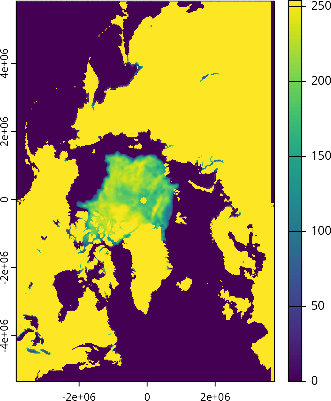
We can turn the data into a raster object using the terra package. The sea ice concentration values are stored in a 448x304 matrix, which we can convert to a raster object.

sic_matrix <- matrix(sic, nrow = 448L, ncol = 304L, byrow = TRUE)

r <- rast(sic_matrix)

plot(r)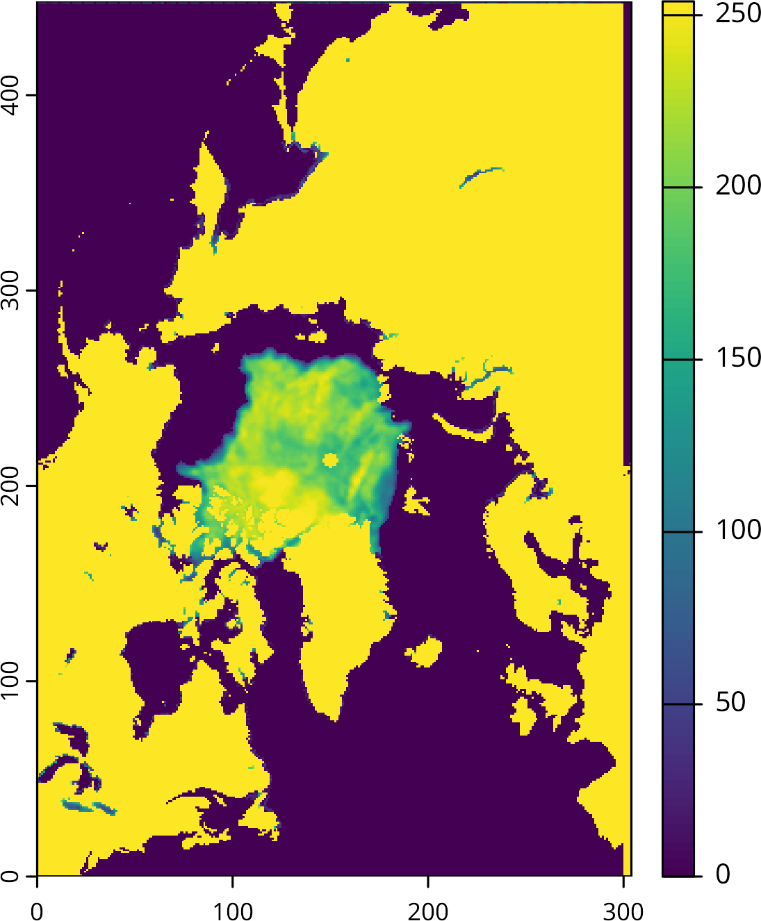

ext(r) <- c(-3850000L, 3750000L, -5350000L, 5850000L)
crs(r) <- "+proj=stere +lat_0=90 +lat_ts=70 +lon_0=-45 +k=1 +x_0=0 +y_0=0 +datum=WGS84 +units=m +no_defs"

plot(r)